SimpleOpt - A General Purpose Optimization Tool (solver) [#1]

[Last updated on: Tuesday, May 12, 2020]

The SimpleOpt algorithm.
Its application to general purpose optimization problems

                            1. Introduction
                            2. A simple example
                            3. The general framework for using the optimizer on user defined problems
                            4. An example of using the general framework for a 2-D function
                            5. Conclusions

                            DOWNLOAD

ABSTRACT

A simple, general purpose optimization tool has been designed and developed under the Python language. The purpose of this document is to describe some practical ways of using this tool from within other Python applications. The introduction (section 1) presents an overview of the category of problems the optimizer is intended for. For making things as attractive and easy understandable as possible, a simple example for the use of the optimizer on a 1-D sine function is provided first (in section 2). Starting from this example, a general framework which can be used as a starting Python script skeleton for other user defined functions is then presented (section 3). Finally, a more complex example, of using the optimizer on a highly customizable 2-D function, using the above framework, is discussed (section 4). This document ends with some conclusions (section 5) and a list of available downloads.

1. Introduction

The optimizer is intended to solve the general category of problems, which we shall try to briefly describe in the following.

Suppose that we have an objective function (F), defined on a subset (S) of the real Euclidean n-dimensional space:

F : S --> R, where S is a subset of Rⁿ.

The subset S, is defined as a n-dimensional interval (a "hyper box"):

S = [x_{0 min}, x_{0
max}] x ... x [x_{i min}, x_{i max}] x ... x [x_{n-1
min}, x_{n-1 max}],

with x_{i min}, x_{i
max} in R.

We have to optimize this function. This means that we should find (ideally) all the points X*, for which the function F has local maxima:

F(X*) = max,

and satisfying some constraints, given by a set of relations in the form of:

G_j(X*) <= 0, where j = 0 ... m - 1, X* in S.

In conclusion, the optimization problem we have to deal with, could be defined by the triplet: space, function, constraints <S, F, G>. In this approach, each of the above elements is procedurally defined. This is an alternative to the symbolic approach, used by other optimization algorithms (such as CONOPT).

The algorithm consists in a simple incremental maximum search procedure in the problem space S (restricted by the constraints G_j), using "flexible" point neighborhoods. It is implemented in Python in the form of two modules named problem.py and simpleopt.py. The detailed implementation of the optimization algorithm is not subject of this document.

(Go to Contents...)

2. A simple example

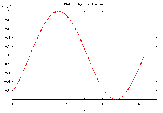
Let's first consider that we want to write a Python application which can solve the concrete 1-D optimization problem of a sine function:

F = sin(x),

defined on:

S = [-0.9, 2pi + 0.1].

A graph of this function is represented in figure 2.1.

Figure 2.1

We want to optimize this function, restraining only to the [0.5, 2pi] interval. This can be expressed by considering the following system of two constraints:

G₀(x) = 0.5 - x < 0, and G₁(x) = x - 2pi < 0.

How can we express this simple optimization problem, using the Python language?

The problem space S, could be specified by a list of tuples (pairs), each containing the bounds (i.e. a minimum value, and a maximum one) for each coordinate. In our case, n = 1, so our list, let's name it mybounds, contains only one tuple:

mybounds = [ (-0.9, 2*math.pi + 0.1) ].

The objective function F, let's name it myeval(x), could be defined like this:

def myeval(x): return math.sin(x[0]).

Please note that the formal parameter x must be a list of coordinates x[0], ..., x[i], ..., x[n-1]. This is why we used the notation x[0] instead of x, for our 1-D example.

The two constraints G₀ and G₁ could be specified as only one function, myconstraint(i, x), like in the following:

def myconstraint(i, x):
# This defines [0.5, 2pi] as the allowed interval

        if i == 0:         # constraint no. 1
            if x[0] > 0.5: return -1
            else: return 1
        elif i == 1:       # constraint no. 2
            if x[0] < 2*math.pi: return -1
            else: return 1
        else: return 1     # any other constraint...

where i indicates the constraint which should be evaluated for the current point x.

Well, things look quite simple until now. It's time to see how the above definitions could be integrated in a working Python module which uses the optimization algorithm implemented in the problem.py and simpleopt.py modules.

First of all, we must import the required functionalities, both from the modules which implement the optimizer, and from other Python modules (libraries).
Then, we have to insert our previously described definitions (the problem space, as a collection of bounds, the objective function, and the constraints).
Finally, we must write the executable part of the module:
    - specifying the optimization problem, and getting an instance of it,
    - creating a personalized instance of the optimizer,
    - executing the above instance of the optimizer (by calling the optsearch method).

The Python program will look like this:

from problem import Problem
from simpleopt import SimpleOpt

import math

# ------------------------------------------------------------------

mybounds = [ (-0.9, 2*math.pi + 0.1) ]

def myeval(x): return math.sin(x[0])

def myconstraint(i, x):
# This defines [0.5, 2pi] as the allowed interval

    if i == 0:         # constraint nr. 1
        if x[0] > 0.5: return -1
        else: return 1
    elif i == 1:       # constraint nr. 2
        if x[0] < 2*math.pi: return -1
        else: return 1
    else: return 1     # any other constraint...

# -------------------------------------------------------------------
# Program starting point
# -------------------------------------------------------------------

if __name__ == "__main__":

    myproblem = Problem("func1d", 1, 2, mybounds, myeval, myconstraint)
    so = SimpleOpt(myproblem, 100000, 0.001, 5, 0, 0)
    so.optsearch()

# -------------------------------------------------------------------
# -------------------------------------------------------------------

Let's explain a little bit more the executable part of the above program.

By calling the class Problem, defined in the problem.py module, the variable myproblem gets an instance of the current optimization problem, defined by: the dimension of the input space (1), the number of constraints (2), the list of bounds (mybounds), the objective function (myeval), and the set of constraints (myconstraint).

By calling the SimpleOpt class, defined in the simpleopt.py module, the variable so gets an instance of the optimizer ready to be applied to our problem (myproblem), and using a maximum number of steps / iterations for the search process (100000), a minimum search step size (0.001), and the option of non-plotting any graphs (0).

The SimpleOpt's class method optsearch starts the searching process for a local maximum.

If the search process succeeds, the maximum value of the objective function, and the point in which it was found, are displayed.

REMARK:

Each run of the optsearch method eventually finds a single local maximum. In order to find all of them, the process should be re-run a number of times. Obviously, this number depends on the topology of the (hyper-)surface representing the graph of the objective function over the problem space. As it is now, the algorithm doesn't guarantee that for each new run, a different maximum will be found. This implies that even if you found the same maximum for a number of successive trials, this doesn't mean that there are no other maxima to be still found. To be somehow sure that (almost) all the maxima have been found, several trials could be necessary for certain objective functions.

In order to run yourself the above Python code, you can:
- either copy and paste the script from this page (as text only) in a simple text file (e.g. func1d.py),
- or, preferably, download the func1d.py script directly from here,
and then use the command:

python func1d.py

Obviously, you should also have the optimizer modules already on your computer. If not, you can download them now (choose one of: the new SimpleOpt for Python 3.x, or the old SimpleOpt for Python <= 2.x).

REMARK:

When running the above program, if the numeric.py and gnuplot.py modules, and the Gnuplot utility, or alternatively, the MatPlotLib library and numpy module are installed on your computer, the optsearch method can also provide a graph representing the evolution of the objective function during the search of a local maximum. Such graphs are represented in Figure 2.2, and 2.3 (and also further in section 4). In each of them, "best solution" at iteration k, means the value of the function for the point considered at step k. The graph always represents an increasing curve. This happens because the search algorithm tries to find points for which the value of the objective function is greater than for the current one, at each step / iteration. The curve depends on the starting search point, and ends either when a real local maximum is found, or the allowed number of steps / iterations is reached, or the domain limit is overridden.

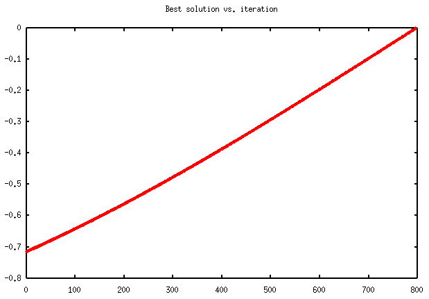
Figure 2.2

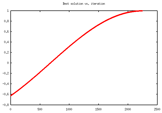
Figure 2.3

The graphs in Figures 2.2 and 2.3, are obtained for two different runs of the program. The first describes a 800 steps process, through which a boundary maximum of value 0 is found in 2pi. The second one, shows a 2250 iterations process, which found the real maximum of the sine function in pi/2.

(Go to Contents...)

3. The general framework for using the optimizer on user defined problems

Having in mind the above simple example (section 2), we can try to define now a general framework for using the optimizer on user defined problems. Such a framework should contain the following parts:

an "import" part, specifying:
- the required classes from the optimizer related modules (mandatory)
- the class(es) and methods from other modules, according to application needs (optional)
a definition part, including:
     - data structures and functions necessary for the definition of the objective function and constraint(s)
     - specification of the problem space: list of bounds on each coordinate, as a tuple (x_min, x_max)
     - the procedure definition for the objective function
     - the procedure definition for the constraint(s)
the executable part, containing:
     - the specification of the optimization problem
     - the instantiation of the optimizer class for the specified problem
     - the start of one optimization process.

The Python-like code implementing these ideas is shown bellow. Please note, that it doesn't really represent a directly executable script as it is. The portions written between '<' and '>' characters should be replaced by the appropriate Python data / function(s), to customize the code according to your application.

# -------------------------------------------------------------------
# Mandatory imports:
# - problem definition class
# - simple, general-purpose optimizer class
# -------------------------------------------------------------------

from problem import Problem
from simpleopt import SimpleOpt

# -------------------------------------------------------------------
# Auxiliary imports
# -------------------------------------------------------------------

import math
#import Numeric # needed only for plotting purposes
#import Gnuplot # needed only for plotting purposes

# -------------------------------------------------------------------
# Auxiliary data and function definitions
# -------------------------------------------------------------------

# -------------------------------------------------------------------
# Specification of the problem space:
# list of bounds on each coordinate, as a tuple (xmin, xmax)
# -------------------------------------------------------------------

mybounds = < list_of_binary_tuples >

# -------------------------------------------------------------------
# Procedural definition of the objective function f
# -------------------------------------------------------------------

def myeval(x):
< objective_function_statements >

# -------------------------------------------------------------------
# Procedural definition of the set of constraints gi
# -------------------------------------------------------------------
# NOTE: Each i personalizes a constraint function gi. For a given i
# (that is, a given constraint, myconstraint(i, x) must return a
# value < 0 if the constraint is satisfied, and > 0 if not
# -------------------------------------------------------------------

def myconstraint(i, x):
    if i == 0:         # constraint nr. 1
        < constraint_1_statements >
    elif i == 1:       # constraint nr. 2
        < constraint_2_statements >
    elif i == 2:       # constraint nr. 3
        < constraint_3_statements >

    ...

    else: return 1     # any other constraint...

# -------------------------------------------------------------------
# Program starting point
# -------------------------------------------------------------------

if __name__ == "__main__":

# Here can be drawn a graph of the objective function

< appropriate_statements >

    # Specify your optimization problem here, getting an instance of
    # it. Parameters:
    #     - problem name
    #     - dimension of the input space
    #     - number of constraints
    #     - list of bounds
    #     - objective function
    #     - constraints function
    #     - desired starting point reference (optional list of coordinates)

    myproblem = Problem(< problem_name >,
                                                < dimension_of_problem_space >,
                        < number_of_constraints >,
                        mybounds,
                        myeval,
                        myconstraint,
                        seedpoint = < value >)

    # Create a personalized instance of the optimizer, by specifying:
    #     - the problem
    #     - maximum number of steps / iterations for the search process
    #     - minimum search step size (the search process resolution)
    #     - maximum search depth (1 - 500)
    #     - whether to use backtracking (1), or not (0)
    #     - whether to use graphics (1), or not (0)

    so = SimpleOpt(myproblem,
                   < number_of_steps >,
                   < minimum_search_step_size >,
                   < maximum_search_depth >,
                   < option_to_use_or_not_backtracking >,
                   < option_to_plot_or_not_graphs >)

# Start the optimizer

so.optsearch()

# -------------------------------------------------------------------
# -------------------------------------------------------------------

REMARKS:

Please note that the parameters of the simpleopt method, referred above as number_of_steps and minimum_step_size, must be chosen according to the concrete problem. They should also be correlated to each other (lesser minimum_step_size requires greater number_of_steps).

The maximum_search_depth parameter could be considered as a measure of the "stubbornness" with which the algorithm tries to find a possible new optimum around the current candidate. Smaller values should be used for problems having relatively smooth objective function, while larger ones are indicated for problems with "spiky" objective function (including the linear programming type ones).

The problem_name parameter is used only for identifying a log file (with the extension .log) which is generated while running the problem associated SimpleOpt instance, and storing most of the information displayed on the screen during this process.

(Go to Contents...)

4. An example of using the general framework for a 2-D function

Based on the framework described in section 3, we present a more complex example, of a 2-D objective function optimization. We consider a real function F, defined on the square [0, 8] x [0, 8], in the form of a sum of exponentials:

                      k
        F(X) = Sum f_i(X)
                     i=1

where,

                                      d(P_i, X)
        f_i(X) = b_i exp( - ------------- )).
                                          a_i

Each exponential f_i is centered on a point P_i, has an amplitude b_i, and a "form factor" given by the parameter a_i. It depends on the current point X = (x₀, x₁), by means of the Euclidean distance d, between the center P_i and X. Each exponential f_i determines a maximum of the objective function F in each point P_i. For the example presented here, we defined a function F, composed of 7 exponentials f_i, and thus having 7 maxima. All exponentials have the same amplitude (b_i = 1) and "form factor" (a_i = 2)

A graph of the above described objective function is depicted in Figure 4.1.

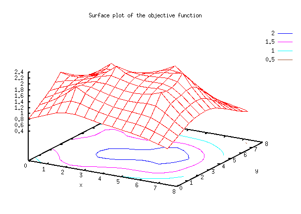
Figure 4.1

Let's consider that the optimization problem we want to solve is subject to a single constraint, representing a circular domain of radius 3, centered in [4, 4].

The Python code which attempts to solve this problem is shown bellow.

from problem import Problem
from simpleopt import SimpleOpt

# -------------------------------------------------------------------
# Auxiliary imports
# -------------------------------------------------------------------

import math
#import Numeric # needed for plotting purposes
#import Gnuplot # needed for plotting purposes

# -------------------------------------------------------------------
# Auxiliary data and function definitions
# -------------------------------------------------------------------

p = [(1, 6), (0, 3), (2, 1), (3, 3), (5, 5), (6, 4), (6, 2)]
alfa = [2, 2, 2, 2, 2, 2, 2]
beta = [1, 1, 1, 1, 1, 1, 1]
center = (4, 4)
radius = 3

def dist(x, y):
return math.sqrt((x[0] - y[0])*(x[0] - y[0]) +
(x[1] - y[1])*(x[1] - y[1]))

def hump(i, x):
return beta[i] * math.exp(-dist(p[i], x) / alfa[i])

# -------------------------------------------------------------------
# Specification of the problem space:
# list of bounds on each coordinate, in the form (xmin, xmax)
# -------------------------------------------------------------------

mybounds = [(0, 8), (0, 8)]

# -------------------------------------------------------------------
# Procedural definition of the objective function f
# -------------------------------------------------------------------

def myeval(x):
    sum = 0
    for i in range(len(p)): sum += hump(i, x)
    return sum

# -------------------------------------------------------------------
# Procedural definition of the set of constraints gi
# -------------------------------------------------------------------
# NOTE: Each i personalizes a constraint function gi. For a given i
# (that is, a given constraint, myconstraint(i, x) must return a
# value <= 0 if the constraint is satisfied, and > 0 if not
# -------------------------------------------------------------------

def myconstraint(i, x):
    if i == 0:            # constraint nr. 1
        return dist(x, center) - radius
    else:
        return 1          # any other constraint...

# -------------------------------------------------------------------
# Program starting point
# -------------------------------------------------------------------

if __name__ == "__main__":

# Here can be drawn a graph of the objective function
# < ... (insert appropriate code) ... >

myproblem = Problem("func2d", 2, 1, mybounds, myeval, myconstraint)

    # Create a personalized instance of the optimizer, by specifying:
    #     - the problem
    #     - maximum number of steps for the search process
    #     - minimum search step size (the search process resolution)
    #     - maximum search depth (1 - 500)
    #     - whether to use backtracking (1), or not (0)
    #     - whether to use graphics (1), or not (0)

so = SimpleOpt(myproblem, 100000, 0.001, 5, 0, 0)

# Start the optimizer

so.optsearch()

# -------------------------------------------------------------------
# -------------------------------------------------------------------

In order to run yourself the above Python code, you can:
- either copy and paste the script from this page (as text only) in a simple text file (e.g. func2d.py),
- or, preferably, download the func2d.py script directly from here,
and then use the command:

python func2d.py

Please remember that on one run, only one maximum is found. To find all of them, several trials should be considered.

Figures 4.2 and 4.3 present the evolution of the searching process at each step, for two different runs.

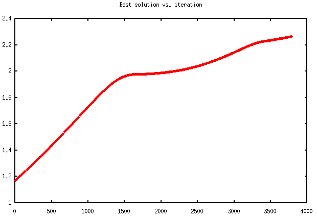
Figure 4.2

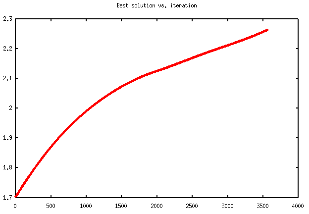
Figure 4.3

REMARK:

The above example could be considered as a good test environment for the optimizer capabilities. The function F could be dramatically modified, by appropriately choosing the number of points P_i, the amplitudes b_i, the "form factors" a_i, and by defining different constraint regions. Perhaps, a good starting point for tests could be to change the radius of the constraint region, and / or the amplitudes of the exponentials.

(Go to Contents...)

5. Conclusions

A simple, general purpose optimization tool has been designed and developed under the Python language. This document described some practical ways of using this tool from within other Python applications. A simple 1-D example, of a sine objective function optimization program was presented and commented first. Starting from this easy to understand example, a general structure for Python applications which use the optimizer has been sketched then. Finally, a more complex program example, built on the above general structure, intended to optimize a 2-D objective function was presented. This last example could be the base for a lot of experiments, the proposed objective function being entirely customizable by its parameters. Thus, the strengths and limitations of the optimizer can be revealed. Using the general framework presented in section 3, one can even experiment the behavior of the optimizer on various real world problems.

(Go to Contents...)

DOWNLOAD:

simpleopt.py	the Python 3.x code for the optimizer module
problem.py	the Python 3.x code for the problem specification
func1d.py	the Python code to call the optimizer for a sine function (1-D example)
func2d.py	the Python code to call the optimizer for a sum of exponentials function (2-D example)
simpleopt.zip	the "zip" archive containing the SimpleOpt modules (for Python 3.x)
simpleopt-old.zip	the "zip" archive containing the SimpleOpt modules (for Python <= 2.x)

(Go to Contents...)

< Go to SimpleOpt main page >